Recursion: where it all began

The tale of dynamic programming all started from recursion, a cousin of iteration. To illustrate the how they can achieve the same thing, let’s imagine that we have a 0-indexed list with $n$ elements:

Let’s start with something simple: let’s get the $k_{th}$ element of the list given the head iterator of the list. Normally, one would start with a while or for loop:

1
2
3
4

iter = head
for i in range(k):
    iter = iter.next()
print("Kth element", iter)

While we are satisfied with the above solution, one can also do it recursively.

1
2
3
4
5
6
7
8

def get_kth_elem(iter, num):
    if num == 0:
        print("Kth element", iter)
        return

    get_kth_elem(iter.next(), num-1)

get_kth_elem(head, k)

The above two procedures accomplish the same thing, but the recursive one is clearly demonstrating it’s true definition:

(Resursion is a method of solving a computational problem where …) the solution to a problem depends on a smaller instance of the same problem.

In the above example, printing the $k_{th}$ element of the whole list is the same as printing the $k-1_{th}$ element of the same list if we start from the second element as the head, an is the same as printing the $k-2_{th}$ element of the same list if we start from the third element as the head, and so on. This thinking process might sound unnecessarily redundant, its beauty will shine once one realizes that it exists in many places in our world.

For now, let’s say that a procedure is recursive if the procedure depends on a smaller instance of the same procedure.

Trees: a recursive data structure

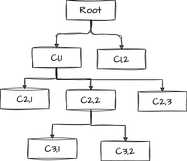
When a construct, or a data structure exhibits the trait similar to a recursive procedure, in which a part of this construct consists of one or more smaller instances of the same construct, we say that the construct is also recursive. A prime example that one in the field of computing often comes up with is a tree. We usually draw a tree from the top to the bottom instead of the other way around.

Why is it recursive? If we view every node and its decendants as a tree, then the root node represents the whole tree. In the above example, its root node has two child nodes $C_{1,1}$ and $C_{1,2}$ with some decendants each, so they are also trees that represent a portion of the whole tree. We call them subtress. Similarly, their children are also subtrees (or sub-subtrees if you are rigorous) of the whole tree, until we reach to a leaf node (i.e., the node without any children) which is the simplest form of a tree.

To construct a tree, we can use a recursive procedure. We start from the top, root node. But, to construct the root node which is the entire tree, we need to construct its children. Then, we go to each of its children, from which we need to go further down to construct their children. In other words, the procedure of constructing the tree consists of some procedures of constructing smaller trees. This procedure is thus recursive. A rather non-rigorous piece of code can be used to perform this procedure:

 1
 2
 3
 4
 5
 6
 7
 8
 9
10

def construct_tree(depth: int):
    node = Node()
    # Suppose we want to stop here as we've reached our desired depth.
    if depth == target_depth:
        return node
    children = []
    for i in range(children_count):
        children.append(construct_tree(depth+1))
    node.children = children
    return node

Interestingly, the visitation procedure to go through every node in a tree is following the same pattern as the construction procedure:

1
2
3
4
5
6
7

def visit(node):
    # We are visiting the current node.
    # For now, let's just print it.
    print(node)
    # Then, visit all children
    for child in node.children:
        visit(child)

Again, to visit the entire tree, we visit every node, from which we visit every child of it - recursively.

A careful reader will notice that for every node, we grow its sub-tree only once. This is due to the nature of a “tree”: for every node, it only has one parent. This means that if we are visiting a node, the only path via which we get led here is through its sole parent. We can extend this logic via induction to prove that using the above recursive procedure visits every node only once.

One would also notice that the very first example of a list, is also a recursive data structure: every element has one predecessor (except the first) and one supercessor (except the last). In fact, we can visit our list in this procedure given an iterator:

1
2
3
4

def visit_list(iter):
    if iter is None:
        return
    visit_list(iter.next())

Now comes the true nature of dynamic programming.

DAG, the true nature of dynamic programming

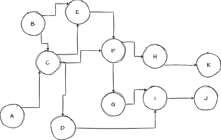
Now, a curious reader would want to know: what if we modify our tree in a way that each node may have more than one parent. Well, it can’t be called as a tree, can it? Such a “tree” doesn’t exist in nature anyways. In fact, in the discipline of Graph Theory, we have another name that generalizes such constructs: Directed Acyclic Graphs (DAGs).

Let’s look at every word in this term and check if a tree exhibits the concept of that term:

1. Directed: a tree is inherently directed - we mentioned that we grow a tree downward (of course, one can grow it upward just like a real tree). There’s no tree that grows backward to its root in nature.
2. Acyclic: it means that there’s no cycle in this graph. A tree by definition cannot have cycles.
3. Graph: a tree is a type of graph/network, a more specific type of graph where 1) we specify the direction to go from one node to another, and 2) that every node has just one (or no) parent, and 3) that the graph has only starting point (the root) from which we can visit all nodes. A DAG is just like a tree, except the fact that a node may have more than one parent, and that the graph may not have a single point from which we can visit all nodes.

Now, if one wishes to perform the visitation of a DAG using the previous procedure, where should she/he start if there’s no single starting point? Well, we’ve got to try every node (possibly as few as one can to save some effort) from which one can visit the entire graph. In the above picture, one would chose $A$ and $B$ as the starting points.

But, if one is cognizant of the cost of using the same recursive pattern as that for a tree, one will see that some nodes will be visited multiple times:

From $A$, we visit $C$, from which we visit $F$, from which we visit $G$, from which we visit $I$, from which we visit $J$; then, from $F$ we visit $H$ then, from which we visit $K$, from which we visit $I$, from which we visit $J$; then, from $C$ we visit $E$, from which we visit $F$, from which we visit $G$, …

This is getting absurdly long, but one can clearly see that several nodes are visited repeatedly. This is particularly problematic if the DAG is huge (large number of nodes / edges). What if we come up with an optimization technique such that one will remember the nodes (or subgraphs) that have been visited when we come to them for the second, third, fourth, … time?

Well, that is what dynamic programming is all about. It’s an optimization technique used to save states that have already been computed to avoid repeated computation. One can come up with the following optimized visitation procedure for a DAG:

 1
 2
 3
 4
 5
 6
 7
 8
 9
10
11
12

visited = {node: False for node in nodes}

def visit(node):
    # Avoid repeated visitation on the same subgraph.
    if visited[node] is True:
        return
    # print the node for now as the "visit" action.
    print(node)
    for neighbor in node.neighbors:
        visit(neighbor)
    # Remember that it has been visited.
    visited[node] = True

Repeated computation is a main source of inefficiency, in both the field of computing and our real life. This is the beauty of dynamic programming - to save repeated efforts in computing.

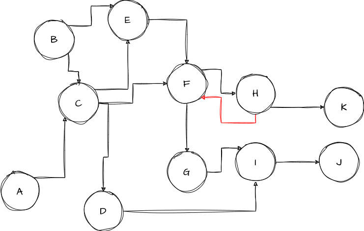
Now, one may ask: what if the graph is cyclic (i.e., has cycles)? Will the above procedure, or dynamic programming work? The answer is: No, unfortunately. To see why it would fail, let’s just add a backward edge from $H$ to $F$ on the DAG, which makes it a non-DAG now:

This graph has a cycle that includes $F$ and $H$. When one visits $F$, she/he would visit $H$ as the next step; however, to complete the visitation on the subgraph represented by $H$, one would need to visit $F$. This recursion will never end. It will dig a infinitely deep hole in your brain; for a poor computer that is running this procedure, its stack space would overflow with recursive calls…

At this point, I will create my own “definition” for dynamic programming as the following:

Dynamic programming is an optimization technique used to remember the visitation of nodes in a DAG such that they won’t be repeatedly visited.

I don’t particularly find the terms frequently appearing in the definition of dynamic programming, such as “optimal substructures” and “subproblems” intuitive. Instead, a DAG can be visualized and reasoned about more easily. Imagine that you are reading “Introduction to Algorithms”, and you look at the steps to develop a dynamic programming algorithm [1]:

1. Characterize the structure of an optimal solution.
2. Recursively define the value of an optimal solution.
3. Compute the value of an optimal solution, typically in a bottom-up fashion.
4. Construct an optimal solution from computed information.

A DAG is an optimal structure because there’s no cycle, implying that repeated visitation is impossible if one saves the computation previously. Every node in a DAG is a optimal solution because the subgraph starting from it is a DAG. While the steps above are absolutely correct and rigorous, if one can effectively translate a problem scenario into a DAG, the above steps can be forgotten completely when developing a dynamic programming procedure.

Now, I’ve come up my own steps for developing a dynamic programming procedure:

1. Understand the problem scenario.
2. Translate the problem scenario into a DAG where each node represents some state, and each edge between two nodes represents the difference in their computed results.
3. Visit the DAG recursively with the extension where states are remembered to avoid repeated computation.

That, is the tale of dynamic programming, where it started from the beautiful concept of recursion, and ends at the abstract but optimal nature of DAGs.

References

[1] T. H. Cormen, C. E. Leiserson, R. L. Rivest, and C. Stein, Introduction to Algorithms. Cambridge, Massachusett: The MIT Press, 2022.